Voxel Cone Tracing

Illumination components

If our scenes only contain point lights (e.g., omni lights, spotlights, etc.) and emissive surfaces, the illumination contributions at a surface position, \(x\), are computed as follows:

1. The self emission associated with the emissive surface (i.e. 0 bounces/surface interactions) is computed as usual without using the scene’s voxelization (as is the case for adding this illumination contribution to the scene’s voxelization);
2. The direct illumination associated with the point lights (i.e. 1 bounce/surface interaction) is computed as usual without using the scene’s voxelization (as is the case for adding this illumination contribution to the scene’s voxelization);
3. The direct illumination associated with the emissive surfaces (i.e. 1 bounce/surface interaction) is obtained from the scene’s voxelization using voxel cone tracing;
4. The indirect illumination associated with the point lights (i.e. 2 bounces/surface interactions) is obtained from the scene’s voxelization using voxel cone tracing.

By computing the diffuse illumination for all the voxels from the scene’s voxelization using voxel cone tracing, the diffuse illumination from additional bounces/surface interactions can be (optionally) accumulated inside the voxels. This requires each voxel to store (an approximation) to the normal distribution of the scene’s surfaces overlapping those voxels as well.

Illumination from the scene’s voxelization (3)-(4)

The outgoing radiance obtained from the scene’s voxelization (\(L_v\)):

For a diffuse BRDF \(f_{r}\!\left(x, \hat\omega_o, \hat\omega_i\right) = \frac{k_d}{\pi}\):

For a partitioning of \(\Omega\) in \(N\) disjunct subdomains, \(\Omega_j\), (e.g., \(\approx\) cones) (i.e. \(\Omega_1 \cup~...~\cup \Omega_N = \Omega\) and \(\Omega_i \cap \Omega_j = \emptyset\) for each \(i \ne j\)):

Relying on a single cone with a direction, \(\hat\omega_{j}\), and an aperture, \(\alpha_{j}\), instead of individual rays with a direction, \(\hat\omega_{j,i}\), for each subdomain, \(\Omega_j\):

We can use for example, the following six cones, each with an aperture of \(\frac{\pi}{6}\).

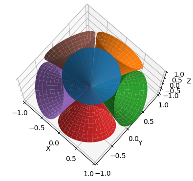
The normalized weight of the blue cone about the surface normal is equal to:

The normalized weight of the other cones is then approximately equal to:

For a specular BRDF, one typically uses a single cone with a direction, \(2 \left(\hat{n} \cdot \hat\omega_o\right) \hat{n}-\hat\omega_o\) (i.e. reflected direction of \(\hat\omega_o\) about \(\hat{n}\)), and an aperture based on the roughness of the surface material.

Voxel Cone Tracing

\(L_v\!\left(x, \hat\omega_{j}, \alpha_{j}\right)\) is computed using voxel cone tracing, which can be implemented by marching the mip-mapped 3D voxel texture in UVW texture space.

Our accumulated radiance (red, green, blue channels) and opacity (alpha channel) are initialized to zero.

Lv ← [0, 0, 0, 0]

Our cone marching distance is initialized to an offset to avoid sampling the self emission associated with the emissive surfaces and the direct illumination associated with the point lights twice. Basically, we need to skip the voxel containing the surface position for which the outgoing radiance needs to be estimated.

distance ← voxel_offset

Marching continues until we reach an accumulated opacity of one or more:

while Lv.alpha < 1:
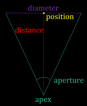
	compute diameter (i.e. cone voxel footprint)
	compute mip_level
	compute position at distance
	if mip_level >= max_mip_level or position ∉ [0,1]^3
	    break
	sample Lv_step(position, mip_level)
	Lv.rgb   ← Lv.rgb   + (1-Lv.alpha) * Lv_step.alpha * Lv_step.rgb // blend equation
	Lv.alpha ← Lv.alpha + (1-Lv.alpha) * Lv_step.alpha
	distance ← distance + diameter // marching
return Lv

References

MOULIN M.: MAGE v0.

MOULIN M.: Specular Voxel Cone Tracing, Internal Presentation, Department of Computer Science, KU Leuven, January 2019.