Partitioning Schemes
Given some geometric primitives in a scene, it is possible to partition and organize these primitives in multiple ways in a hierarchical or non-hierarchical data structure to exploit spatial coherence during ray tracing. We can partition the geometric primitives into two or more disjoint groups without taking the scene (explicitly) into consideration during the partitioning itself. Or we can do the complete opposite by partitioning the scene’s space into two or more disjoint groups without taking the geometric primitives (explicitly) into consideration during the partitioning itself. Or we can use a combination of these two extremes. More formerly:
- Spatial partitioning schemes (recursively) subdivide a given space into spatially disjoint groups. This makes an efficient ray traversal possible at the expense of referencing geometric primitives multiple times.
- Object partitioning schemes (recursively) subdivide a given set of geometric primitives into disjoint groups which tightly comprise their geometric primitives. Geometric primitives are referenced just once at the expense of a less efficient ray traversal in case of spatially overlapping groups.
- Hybrid partitioning schemes combine both spatial and object partitioning schemes.
For closest-hit ray queries (e.g., camera rays, indirect rays, etc.), we want to find the closest hit point of rays with the scene. Therefore, the most efficient traversal of a ray through the acceleration data structure is a front-to-back ray traversal. Such a traversal is trivially to achieve for spatial partitioning schemes, but not for object partitioning schemes due to the possible spatial overlapping between the different groups of geometric primitives.
Any-hit ray queries (e.g., shadow rays) do not care about the closest hit point, any hit point will do. The efficient traversal of any-hit queries, however, is a completely different story beyond the scope of this post.
Acceleration Data Structures for Ray Tracing
Various acceleration data structures exist for exploiting spatial coherence during ray tracing. The faster these structures can be traversed and the less geometric primitives that need to be tested for intersection by rays, the more effective these structures are. Currently, the most effective acceleration data structures are hierarchical, adaptive tree structures of which the leaf nodes reference the geometric primitives and the internal nodes contain spatial information (i.e. splitting plane position, bounding box) to cull the associated part of the scene.
I will give a short overview of some of these structures, and more particularly the considered candidate partitions. Assuming a top-down tree construction, we start with a voxel containing all the geometric primitives that need to be partitioned, and an associated AABB (e.g., the AABB of the complete scene or the AABB of a highly tessellated model). We typically propose a certain number of candidate partitions for the current parent voxel which consists of all child voxels (i.e. the AABB constituting the voxel and the geometric primitives contained in that voxel). We select the best one according to some heuristic/cost function (e.g., SAH) and then decide whether we apply that best candidate partition (i.e. create an intermediate node) or not (i.e. create a leaf node).
As we will see, the structure of these candidate partitions differ between different acceleration data structures. But in all cases, a candidate partition is completely determined given a parent voxel and a splitting plane. For object partitioning schemes, the geometric primitives are mapped to their centroids (or another point) to determine the positioning relative to the splitting plane.
(Binary) Space Partition - BSP
- spatial partitioning scheme
- hierarchical
- binary/n-ary tree
- (non-)axis-aligned voxels
In case of a binary tree with axis-aligned voxels, the BSP is called a kd-tree or rectilinear BSP.
Geometric primitives of the child voxels
- Geometric primitives whose AABB is to the left of the splitting plane belong to the left child voxel.
- Geometric primitives whose AABB is to the right of the splitting plane belong to the right child voxel.
- Geometric primitives whose AABB is straddling the splitting plane belong to both child voxels.
AABBs of the child voxels
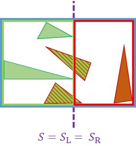
The AABB of both child voxels can be trivially computed given the parent voxel and the splitting plane. The spatial union of the AABB of both child voxels is equal to the parent voxel (none of the six surrounding planes is tight).
Split clipping is a possible optimization (i.e. clipping the geometric primitives against the splitting plane and/or the AABB of the parent voxel). It is possible that the AABB of a geometric primitive straddles the splitting plane, but the actual geometric primitive only lies on one side of the splitting plane. It is even possible that the AABB of a geometric primitive overlaps with a parent voxel, but not the geometric primitive associated with this AABB.
Geometric primitives of the child voxels
- Geometric primitives to the left of the splitting plane belong to the left child voxel.
- Geometric primitives to the right of the splitting plane belong to the right child voxel.
- Geometric primitives straddling the splitting plane belong to both child voxels.
- Geometric primitives lying outside the parent voxel belong to none of the child voxels.
AABBs of the child voxels
The AABB of both child voxels can be trivially computed given the parent voxel and the splitting plane. The spatial union of the AABB of both child voxels is equal to the parent voxel (none of the six surrounding planes is tight).
- (+) \(\mathcal{O}\left(N \log N\right)\) full sweeping-plane SAH build algorithm is possible for constructing complete BSPs.
- (+) \(\mathcal{O}\left(N \log N\right)\) binned SAH build algorithm for constructing complete BSPs (in parallel) is possible.
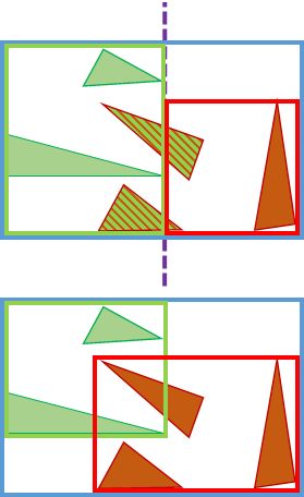
While observing the image of a BSP candidate partition, we clearly see the AABBs associated with the parent, left and right child voxel. A candidate partition is, however, only a conceptual thing to compare different acceleration data structures against each other. The obtained BSPs and kd-trees after construction do not store the AABBs associated with each node. First of all, this would increase the memory footprint. Assume that an AABB consists of 6x 32-bit floating point values (24 bytes) and we have \(2^{30}\) nodes. This results in 24 Gbytes for the AABBs alone. This is clearly something we want to avoid given that BSPs already suffer from high memory usage due to reference duplication for geometric primitives straddling a splitting plane. Furthermore, if we really wanted the AABB of a particular node, we can construct it starting from the AABB of the root node (this is the only AABB we explicitly store) and the splitting planes (i.e. split position and split axis) found along the way while traversing the tree from the root node to our target node. So how do we traverse such a tree without AABBs? We just start at the root node and test the ray for intersection with the splitting plane. Depending on the result, we only need to traverse the left, right or both child voxels in front-to-back order along the ray. This ray-plane intersection test is also much cheaper than a ray-AABB intersection test.
References
BENTLEY J. L., FRIEDMAN J. H.: Data Structures for Range Searching. ACM Comput. Surv. 11, 4 (Dec 1979), 397–409.
IZE T., WALD I., PARKER S. G.: Ray tracing with the BSP tree. In IEEE Symposium on Interactive Ray Tracing 2008 (Aug 2008), pp. 159–166.
KAPLAN M. R.: The Use of Spatial Coherence in Ray Tracing. ACM SIGGRAPH Course Notes 11 (1985).
Bounding Volume Hierarchy - BVH
- object partitioning scheme
- hierarchical
- binary/n-ary tree
- (non-)axis-aligned voxels
- 6 planes of the voxels are tight
Geometric primitives of the child voxels
- Geometric primitives whose centroid is to the left of the splitting plane belong to the left child voxel.
- Geometric primitives whose centroid is to the right of the splitting plane belong to the right child voxel.
- Geometric primitives whose centroid lies on the splitting plane are added to the left child voxel.
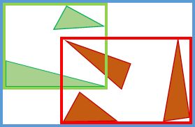
AABBs of the child voxels
The AABB of both child voxels is made tight to the geometric primitives. Note that the AABBs of the child voxels may not be larger than the AABB of the parent voxel, which can occur while constructing SBVHs. In this case, only the overlap with the AABB of the parent voxel will be used.
- (+) \(\mathcal{O}\left(N \log N\right)\) full sweeping-plane SAH build algorithm is possible for constructing complete BVHs.
- (+) \(\mathcal{O}\left(N \log N\right)\) binned SAH build algorithm for constructing complete BVHs (in parallel) is possible.
BVHs are traversed by testing the ray for intersection with the AABBs associated with the intermediate/child voxels.
References
RUBIN S. M., WHITTED T.: A 3-dimensional Representation for Fast Rendering of Complex Scenes. SIGGRAPH Comput. Graph. 14, 3 (Jul 1980), 110–116.
Bounding Interval Hierarchy - BIH
- hybrid partitioning scheme
- hierarchical
- binary/n-ary tree
- (non-)axis-aligned voxels
- 1 plane of the voxels is tight
BIHs are also known as Spatial Kd trees (SKds) and Bounded Kd trees (B-Kds).
Geometric primitives of the child voxels
- Geometric primitives whose centroid is to the left of the splitting plane belong to the left child voxel.
- Geometric primitives whose centroid is to the right of the splitting plane belong to the right child voxel.
- Geometric primitives whose centroid lies on the splitting plane are added to the left child voxel.
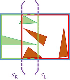
AABBs of the child voxels
The AABB of both child voxels is similar to those of BSPs except that the AABB’s plane corresponding to the splitting plane is made tight to the geometric primitives.
- (+) \(\mathcal{O}\left(N \log N\right)\) full sweeping-plane SAH build algorithm is possible for constructing complete BIHs.
- (+) \(\mathcal{O}\left(N \log N\right)\) binned SAH build algorithm for constructing complete BIHs (in parallel) is possible.
References
HAVRAN V., HERZOG R., SEIDEL H.-P.: On the Fast Construction of Spatial Hierarchies for Ray Tracing. In IEEE Symposium on Interactive Ray Tracing 2006 (Sept 2006), pp. 71–80.
OOI B. C., MCDONELL K. J., RON S.-D.: Spatial Kd-Tree: An Indexing Mechanism for Spatial Databases. In Proceedings of the IEEE COMPSAC Conference (1987).
WÄCHTER C., KELLER A.: Instant Ray Tracing: The Bounding Interval Hierarchy. In Proceedings of the 17th Eurographics Conference on Rendering Techniques (Aire-la-Ville, Switzerland, Switzerland, 2006), EGSR ’06, Eurographics Association, pp. 139–149.
WOOP S., MARMITT G., SLUSALLEK P.: B-Kd Trees for Hardware Accelerated Ray Tracing of Dynamic Scenes. In Proceedings of the 21st ACM SIGGRAPH/EUROGRAPHICS Symposium on Graphics Hardware (New York, NY, USA, 2006), GH ’06, ACM, pp. 67–77.
Note that the papers introducing SKds, B-Kds and BIHs in computer graphics are all from the same year which explains the various synonyms.
GK-BVH
- spatial partitioning scheme
- hierarchical
- binary/n-ary tree
- (non-)axis-aligned voxels
- 6 planes of the voxels are tight, but constrained by the splitting plane
Geometric primitives of the child voxels
- Geometric primitives to the left of the splitting plane belong to the left child voxel.
- Geometric primitives to the right of the splitting plane belong to the right child voxel.
- Geometric primitives straddling the splitting plane belong to both child voxels.
- Geometric primitives lying outside the parent voxel belong to none of the child voxels.
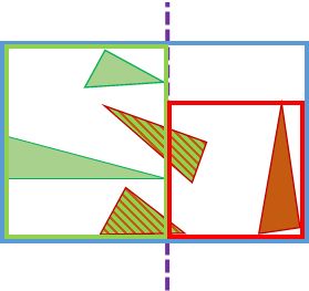
AABBs of the child voxels
The AABBs of the child voxels are made tight to the geometric primitives, but the plane corresponding to the splitting plane can only be moved to the left (right) for the left (right) child voxel. So the geometry first needs to be clipped against the splitting plane. Furthermore, only the overlap with the AABB of the parent voxel will be used when geometric primitives straddle the AABB of the parent voxel.
Originally, I discovered the GK-BVH myself independently and called it a Tight BSP (TBSP) due to its close resemblance to BSPs with regard to the construction. The traversal algorithm, however, is similar to a BVH, explaining the GK-BVH name. The only difference is that geometric primitives can now be associated with multiple leaf nodes and thus the same geometric primitives can be tested multiple times for intersection by the same ray (without using optimizations such as mailboxing). This also implies that the resulting GK-BVH will look differently internally as opposed to BVHs, where the latter can just reorganize the geometric primitives in place and the former will depend on an extra indirection (i.e. indices).
- (-) \(\mathcal{O}\left(N \log N\right)\) full sweeping-plane SAH build algorithm is not possible for constructing complete GK-BVHs due to the involved clipping operations.
- (+) \(\mathcal{O}\left(N \log N\right)\) binned SAH build algorithm for constructing complete GK-BVHs (in parallel) is possible.
We can also clip the AABBs instead of the geometric primitives, which is similar to the difference between kd-trees built with and without split clipping.
Geometric primitives of the child voxels
- Geometric primitives whose AABB is to the left of the splitting plane belong to the left child voxel.
- Geometric primitives whose AABB is to the right of the splitting plane belong to the right child voxel.
- Geometric primitives whose AABB is straddling the splitting plane belong to both child voxels.
AABBs of the child voxels
The AABBs of the child voxels are made tight to the AABBs of the geometric primitives, but the plane corresponding to the splitting plane can only be moved to the left (right) for the left (right) child voxel. Furthermore, only the overlap with the AABB of the parent voxel will be used when geometric primitives straddle the AABB of the parent voxel.
- (+) \(\mathcal{O}\left(N \log N\right)\) full sweeping-plane SAH build algorithm is possible for constructing complete GK-BVHs due to the involved clipping operations.
- (+) \(\mathcal{O}\left(N \log N\right)\) binned SAH build algorithm for constructing complete GK-BVHs (in parallel) is possible.
GK-BVHs are, however, tighter since they perform clipping operations on the geometric primitives (and thus not on their less tighter AABBs). Therefore, GK-BVHs will typically have a smaller geometric reference duplication. The only benefit of not clipping the geometric primitives, but the AABBs instead, is a faster build algorithm and the potential of still being able to use a full sweeping-plane SAH build algorithm in a similar fashion to the way BVHs can be built. The traversal will however be the same as for the GK-BVH, and will thus be the same as for the BVH as well. And the traversal of the latter is more efficient in case of less overlap between the AABBs of the child voxels. Since the tightness of GK-BVHs is larger than your acceleration data structure, GK-BVHs will outperform them.
References
POPOV S., GEORGIEV I., DIMOV R., SLUSALLEK P.: Object Partitioning Considered Harmful: Space Subdivision for BVHs. In Proceedings of the Conference on High Performance Graphics 2009 (New York, NY, USA, 2009), HPG ’09, ACM, pp. 15–22.
Spatial Split Bounding Volume Hierarchy - SBVH
- hybrid partitioning scheme
- hierarchical
- binary/n-ary tree
- (non-)axis-aligned voxels
- combination of BVH and GK-BVH candidate partitions
SBVHs are built with a combination of BVH and GK-BVH candidate partitions.
- (-) \(\mathcal{O}\left(N \log N\right)\) full sweeping-plane SAH build algorithm is not possible for constructing complete SBVHs due to the inclusion of GK-BVH candidate partitions (see above).
- (+) \(\mathcal{O}\left(N \log N\right)\) binned SAH build algorithm for constructing complete SBVHs (in parallel) is possible.
Since, GK-BVHs will be traversed similarly to BVHs, nothing is stopping us from combining GK-BVH and BVH candidate partitions. The original goal was including some spatial splitting in the BVH construction to have the best of both worlds: the compactness of BVHs and the spatial awareness of BSPs. The best BVH candidate partition and the best BSP candidate partition are found per split decision; both using their variant of the SAH. But how do we select the best of these two to obtain one best candidate partition? If we just compare the SAH costs, the BVH candidate partition will be selected in nearly all cases and we end up with a BVH acceleration data structure. Since, the child voxels of a BVH candidate partition are tight which is not the case for the child voxels of a BSP candidate partition, the SAH cost will be lower since the surface area of the child voxels will be smaller. The solution is to make the BSP candidate partition as tight as possible. This way we obtain the GK-BVH candidate partition, which allows for a fairer comparison against BVH candidate partitions (compared to BSP candidate partitions).
Besides being a hybrid of BVH and GK-BVH candidate partitions, the SBVH is more flexible than a GK-BVH. The best candidate partition can be refined if geometric primitives are contained in both child voxels. Each such primitive can be added to the left, right or both child voxels. After iterating these geometric primitives, we obtain the final best candidate partition for a single split decision.
If we do not use optimizations such as LBVHs which uses spatial Morton coding to organize the BVH. The SBVH is conceptually the most effective acceleration data structure presented here so far, offering the best of both worlds (i.e. hybrid of spatial and object partitioning schemes). SBVHs were the preferred acceleration data structure of the NVidia OptiX Ray Tracing Engine.
References
STICH M., FRIEDRICH H., DIETRICH A.: Spatial Splits in Bounding Volume Hierarchies. In Proceedings of the Conference on High Performance Graphics 2009 (New York, NY, USA, 2009), HPG’09, ACM, pp. 7–13.
Note that the papers introducing GK-BVHs and SBVHs are both of the same year and the same conference which explains the implicit inclusion of GK-BVHs in SBVHs without referring to the paper about GK-BVHs.
General Reference
MOULIN M., DUTRÉ P.: On the use of Local Ray Termination for Efficiently Constructing Qualitative BSPs, BIHs and (S)BVHs, The Visual Computer, Volume 35, Issue 12, pp.1809–1826, December 2019 (First online: July 2018).